There was an interesting post and discussion on the NBA subreddit of Reddit on the Hot Hand phenomenon and whether or not it is a fallacy.
A Numberphile video on the topic:
An article on the topic:
https://www.scientificamerican.com/article/do-the-golden-state-warriors-have-hot-hands/
In some parts of the Numberphile video, Professor Lisa Goldberg emphasizes that issues of the “Law of Small Numbers,” which is described in the Scientific American article as:
Early in their careers, Amos Tversky and Daniel Kahneman considered the human tendency to draw conclusions based on a few observations, which they called the ‘‘law of small numbers’’.
when looking at the hot hand phenomenon, comes from the fact that we don’t get to see what happens after an H at the end of a sequence. Let a sequence be a string of shots of some length. A shot is either a make H or a miss T. So a sequence of 3 shots might be:
$$ HTH $$
A make, a miss, and then a make. So looking at that, we see that after the first H, we missed, which is evidence against the hot hand. We don’t care what happens after a miss, the T. We can’t see what happens after the last shot, which is a make. This is what’s noted as causing the “Law of Small Numbers.”
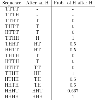
A moment from the Numberphile video illustrating the probabilities of H after an H for each possible sequence of 3 shots, and the average of those probabilities:

And here, this “Law of Small Numbers” causes the average probability of H’s after an H to be 2.5/6. When the sequence is a finite length, the probability of an H after an H (or a T after a T) is biased below 0.5. As the sequence gets longer and tends toward infinity, the probability of an H after an H (or a T after a T) goes toward 0.5.
While all this is true, let’s look a little closer at what’s going on in this illustration to understand why and how exactly this bias occurs.
All possibilities of sequences of 3 shots:
$$ n = \textrm{3} $$

$$ \textrm{Average probability} = \frac{2.5}{6} = 0.416\bar{6} $$
Assuming that an H and a T each appear with 0.5 probability and there is no memory, i.e. no hot hand, each of the above 8 sequences are equally probable. The average probability of the 6 cases where we can evaluate where there is a hot hand or not (cases that have an H in the first or second shot) is calculated to be 2.5/6 < 0.5. But let’s count the number of H’s and T’s in the second column. There are 4 H’s and 4 T’s! So we have:
$$ \frac {\textrm{Number of H’s}}{\textrm{Number of H’s & T’s}} = \frac {4}{8} = 0.5 $$
So it’s as if we’ve undercounted the cases where there are 2 shots that are “hot hand evaluations,” the last two sequences at the bottom of the list. In all (8) sequences of length 3, how many hot hand evaluations in total were there? (How many H’s or T’s in the 2nd column?) 8. How many of those were H’s? 4. So we have a hot hand make probability of 0.5.
It doesn’t necessarily mean that the way they counted hot hand makes in the Numberphile video is wrong. It’s just a particular way of counting it that causes a particular bias. It also may be the particular way the human instinct feels hot handedness – as an average of the probability of hot hand makes over different sequences. In other words, that way of counting may better model how we “feel” or evaluate hot handedness in real world situations.
So why is the average probability over sequences < 0.5?
When we evaluate hot-handedness, we are looking at shots that come after an H. Suppose we write down a list or table of each possible permutation of shot sequences of length \(n\) from less H’s, starting from the sequence of all T’s, down to more H’s, ending with the sequence of all H’s. We noted above that if we count all the hot hand makes H’s in all sequences (the H’s in the 2nd column), the probability of hot hand H’s among all hot hand evaluations (the number of H’s or T’s in the 2nd column) is 1/2. When we look at the list of sequences, what we notice is that a lot of the hot hand H’s (the 2nd column) are concentrated in the lower sequences toward the bottom. But these sequences heavy in so many H’s only give one probability entry in the 3rd column of 1 or near 1.
$$ n = \textrm{4} $$
$$ \textrm{Average probability} = \frac{5.6\bar{6}}{14} \approx 0.405 $$
$$ n = \textrm{5} $$

$$ \textrm{Average probability} = \frac{12.25}{30} \approx 0.408\bar{3} $$
Assuming equal probability of H and T on any given shot and no memory between shots: the entire list of sequences (the 1st column) will have an equal number of H’s and T’s. Additionally, all the hot hand evaluations (the 2nd column) will have an equal number of H’s and T’s.
Looking at the 1st column, we go from more T’s at the top to more H’s at the bottom in a smooth manner. Looking at the 2nd column though, we go from rows of T’s and as we go down we find that a lot of H’s are “bunched up” towards the bottom. But remember that we have a “limited” number of H’s in the 2nd column as well, namely 50% of all hot hand evaluations are H’s and 50% are T’s.
Let’s look closely at how the pattern in the 1st column causes more H’s to be bunched up in the lower sequences in the 2nd column, and also if there is any pattern to the T’s when we look across different sequences.
Higher sequences have less H’s (looking at the 1st column), which means more HT’s in those sequences as well, i.e. more hot hand misses. Lower sequences have more H’s, which means more HH’s in those sequences, i.e. more hot hand makes. This means that, looking at the 2nd column, higher sequences have more T’s and lower sequences have more H’s. Lower sequences “use up” more of the “limited amount” of H’s (limited because the number of H’s and T’s in the 2nd column are equal). Thus, H’s in the 2nd column are “bunched up” in the lower sequences as well. This causes there to be less sequences with higher probability (the 3rd column) than sequences with lower probability. Perhaps this is what brings the average probability below 0.5.
A naive look of the 2nd column shows that the highest sequences have a lone T as its hot hand evaluation, and many other hot hand evaluations of higher sequences end with a T. This makes sense since if a sequence consists of a lot of T’s, any H’s in it are unlikely to be the last two shot in the sequence, like …HH, which is what’s needed for the hot hand evaluations in the 2nd column to end with an H. And as long as a T is the last shot, the hot hand evaluation of the sequence will end with a T, since any lone H or streak of H’s in the sequence will have encountered a T as the next shot either with that last T shot in the sequence (…HHT) or meeting the first of consecutive T’s that lead up to the last T shot of the sequence (…HHTT…T).
Let’s divide up all the sequences in the 1st column into categories of how a sequence ends in its last 2 shots and use that to interpret what the last hot hand evaluation will be in the 2nd column for that sequence category. There are 4 possible ways to have the last 2 shots: TT, TH, HT, and HH. If a sequence ends in …TT, that “…” portion is either all T’s or if it has any H’s, we know that that sequence ends in a T before or at the second-to-last T in the sequence (either …H…TTT or …HTT). So in all cases but one (where the entire sequence is T’s and so there is no hot hand evaluation for the 2nd column), the last hot hand evaluation in the 2nd column will be a T. If a sequence ends in …TH, the thinking is similar to the case that ends in …TT since the very last H doesn’t provide us with an additional hot hand evaluation since the sequence ends right there, so the 2nd column also ends in a T. If a sequence ends in …HT, the last T there is our last hot hand evaluation, so the 2nd column also ends in a T. If a sequence ends in …HH, then the 2nd column ends in an H. So about 3/4 of all sequences end their 2nd column with a T. (\(3/4)n-2\) to be exact, since the sequences of all T’s and \((n-1)\) T’s followed by an H don’t have any hot hand evaluations.) Thus, the T’s in the 2nd column are “spread out more evenly” across the different sequences since (\(3/4)n-2\) of all sequences have a T for its last hot hand evaluation (the 2nd column), while the H’s are “bunched up” in the lower sequences. Thus, a relatively large number of sequences, especially sequences that are higher up, have their probabilities (the 3rd column) influenced by T’s in the 2nd column, bringing the average probability across sequences down.
$$ n = \textrm{6} $$

$$ \textrm{Average probability} \approx 0.4161 $$
As \( n \) grows larger, the average probability seems to drift up.
Looking at the top of the list of sequences for \( n = 4 \), there are 3 sequences with a 0 in the 3rd column. These 3 sequences consist of 1 H and 3 T’s (and TTTH is uncounted because there is no hot hand evaluation in that sequence). At the bottom, we have the HHHH sequence giving a 1 in the 3rd column, and then 4 sequences that have 3 H’s ant 1 T. The entries in the 3rd column for these 4 sequences are 1, 0.5, 0.5, and 0.667.
For sequences of \( n = 5 \), there are then 4 sequences at the top of the list that give a 0 in the 3rd column. At the bottom, the HHHHH sequence gives a 1 in the 3rd column, and then the sequences with 4 H’s and 1 T give 1, 0.667, 0.667, 0.667, 0.75 in the 3rd column.
For sequences of \( n = 6 \), there are then 5 sequences at the top of the list that give a 0 in the 3rd column. At the bottom, the HHHHHH sequence gives a 1 in the 3rd column, and then the sequences with 5 H’s and 1 T give 1, 0.75, 0.75, 0.75, 0.75, 0.8 in the 3rd column.
This pattern shows that as \( n \) increases, we get \( (n – 1) \) sequences at the top of the list that always give 0’s in the 3rd column. At the bottom there is always 1 sequence of all H’s that gives a 1 in the 3rd column. Then for the sequences with \( (n – 1) \) H’s and 1 T, we always have 1 sequence of THH…HH that gives a 1 in the 3rd column, then \( (n – 2) \) sequences that give a \( \frac{n – 3}{n – 2} \) in the 3rd column, and always 1 sequence of HH…HT that gives a \( \frac{n – 2}{n – 1} \) in the 3rd column. So as \( n \) becomes large, the entries in the 3rd column for these sequences with \( (n – 1) \) H’s and 1 T get closer to 1. For small \(n\), such as \(n = 3\), those entries are as low as 0.5 and 0.667. But the entries in the 3rd column for the sequences high in the list with 1 H and \( (n – 1) \) T’s remain at 0 for any \(n\). Thus, as \( n \) becomes large, the lower sequence entries in the 3rd column become larger, shifting the average probability over sequences up.
Roughly speaking, when we only have one shot make in a sequence of shots (only 1 H among \(n-1\) T’s), we have only one hot hand evaluation possible, which is the shot right after the make. Ignoring the case of TT…TH, that hot hand evaluation coming after the H will always be a miss. Thus, when there is only one shot make in a sequence, the hot hand probability is always 0. On the other hand, when we have only one shot miss in a sequence, ignoring the TH…HH case, we will have 1 hot hand miss and many hot hand makes. Thus, our hot hand probability in these sequences with only 1 T will always be less than 1, and approaches 1 as \( n \) approaches \( \infty \). In a rough way, this lack of balance between the high sequences and low sequences drags down the average probability over the sequences below 0.5, with the amount that’s dragged down mitigated by larger and larger \( n \).
A possible interesting observation or interpretation of this is how it might lead to the human mind “feeling” the gambler’s fallacy (e.g. consecutive H’s means a T “has to come” soon) and the hot hand fallacy (e.g. consecutive H’s means more H’s to come). The above results show that in finite length sequences, when a human averages in their mind the probability of hot hand instances across sequences, i.e. across samples or experiences, the average probability is < 0.5. In other words, across experiences, the human mind "feels" the gambler's fallacy, that reversals after consecutive results are more likely. But when a human happens to find themselves in one of the lower sequences on a list where there are relatively more H's than T's in the 1st column, what happens is that the hot hand evaluations (the 2nd column) are likely to have a lot more H's than what you'd expect, because H's are "bunched up" towards the bottom of the 2nd column. What you expect are reversals - that's what "experience" and the gambler's fallacy that results from that experience tells us. But when we find ourselves in a sequence low in the list, the hot hand instances (the 2nd column) give us an inordinately high number of hot hand makes because H's are bunched up towards the bottom of the list. So when we're hot, it feels like we're really hot, giving us the hot hand fallacy. An actually rigorous paper on this subject, also found in a comment from the Reddit post, is Miller, Joshua B. and Sanjurjo, Adam, Surprised by the Gambler’s and Hot Hand Fallacies? A Truth in the Law of Small Numbers. One of the proofs they present is a proof that the average probability of hot hand makes across sequences is less than the standalone probability of a make (i.e. using our example, the average of the entries in the 3rd column is less than 0.5, the probability of an individual make).
Let
$$ \boldsymbol{X} = \{X_i\}_{i=1}^n $$
be a sequence of 0’s and 1’s that is \(n\) long. An \( X_i = 0 \) represents a miss and an \( X_i = 0 \) represents a make.
From the sequence \( \boldsymbol{X} \), we excerpt out the hot hand evaluations, which are shots that occur after \( k \) made shots. In our example, we are just concerned with \( k = 1\). The hot hand evaluation \(i\)’s are
$$ I_k( \boldsymbol{X} ) := \{i : \Pi_{j=i-k}^{i-1} X_j = 1\} \subseteq \{k+1,…,n\} $$
So \( I_k( \boldsymbol{X} ) \) is defined to be the \( i \)’s where the product of the \(k\) preceding \(X\)’s is 1, and \(i\) can only be from among \( {k+1,…,n} \). So for example, let \(k=2\) and \(n=6\). Then firstly, an \(i\) that is in \( I_k(\boldsymbol{X} \) can only be among \( {3,4,5,6} \) because if \(i = 1,2\), there aren’t enough preceding shots – we need 2 preceding shots made to have the \(i\)th shot be a hot hand evaluation. Ok, so let’s look at \(i = 4\). Then,
$$ \Pi_{j=4-2}^{4-1} X_j = X_2 \cdot X_3 $$
This makes sense. If we are looking at \(i = 4\), we need to see if the 2 preceding shots, \(X_2\) and \(X_3\) are both 1.
The theorem stated in full is:
Let
$$ \boldsymbol{X} = \{X_i\}_{i=1}^n $$
with \( n \geq 3 \) be a sequence of independent (and identical) Bernoulli trials, each with probability of success \( 0 \lt p \lt 1 \). Let
$$ \hat{P}_k(\boldsymbol{X}) := \sum_{i \in I_k(\boldsymbol{X})} \frac{X_i}{|I_k(\boldsymbol{X})|} $$
Then, \( \hat{P} \) is a biased estimator of
$$ \mathbb{P} ( X_t = 1 | \Pi_{j=t-k}^{t-1} X_j = 1 ) \equiv p $$
for all \(k\) such that \(1 \leq k \leq n – 2\). In particular,
$$ \mathbb[E] \left[ \hat{P}_k (\boldsymbol{X}) | I_k(\boldsymbol{X}) \neq \emptyset \right] \lt p $$
We have the \(n \geq 3 \) because when \( n = 2 \), we actually won’t have the bias. We have HH, HT, TH, TT, and if \( p = 1/2 \), we have the HH giving us a hot hand evaluation of H and the HT giving us a hot hand evaluation of T, so that’s 1 hot hand make out of 2 hot hand evaluations, giving us the \( \hat{P} = 1/2 \) with no bias.
We have \( \hat{P}_k( \boldsymbol{X} ) \) as our estimator of the hot hand make probability. It’s taking the sum of all \(X_i\)’s where \(i\) is a hot hand evaluation (the preceding \(k\) shots all went in) and dividing it by the number of hot hand evaluations – in other words, the hot hand makes divided by the hot hand evaluations. Note that we are just looking at one sequence \( \boldsymbol{X} \) here.
\( \mathbb{P} (X_t = 1 | \Pi_{j=t-k}^{t-1} X_j = 1 ) \equiv p \) is the actual probability of a hot hand make. Since we are assuming that the sequence \( \boldsymbol{X} \) is \(i.i.d.\), the probability of a hot hand make is the same as the probability of any make, \(p\).
\(k\) is restricted to \(1 \leq k \leq n – 2\) since if \(k = n – 1 \) then the only possible hot hand evaluation is if all first \(n-1\) shots are made. Then we would just be evaluating at most 1 shot in a sequence, the last shot. Similar to the case above where \(n=2\), the estimator would be unbiased. if \(k = n\), then we would never even have any hot hand evaluation, as all shots made would simply satisfy the condition for the next shot to be a hot hand evaluation, where the next shot would be the \(n+1\)th shot.
\( E \left[ \hat{P}_k (\boldsymbol{X}) | I_k(\boldsymbol{X}) \neq \emptyset \right] \lt p \) is saying that the expectation of the estimator (given that we have some hot hand evaluations) underestimates the true \(p\).
Here is the rigorous proof provided by the paper in its appendix:
First,
$$ F:= \{ \boldsymbol{x} \in \{ 0,1 \}^n : I_k (\boldsymbol{x}) \neq \emptyset \} $$
\(F\) is defined to be the sample space of sequences \(\boldsymbol{x}\) where a sequence is an instance of \(\boldsymbol{X}\) that is made up of \(n\) entries of either \(0\)’s or \(1\)’s and there is a non-zero number of hot hand evaluations. In other words, \(F\) is all the possible binary sequences of length \(n\), like the lists of sequences we wrote down for \(n = 3,4,5,6\) above. By having \( I_k (\boldsymbol{x}) \neq \emptyset \), we have that \( \hat{P}_k(\boldsymbol{X}) \) is well-defined.
The probability distribution over \(F\) is given by
$$ \mathbb{P} (A|F) := \frac{ \mathbb{P} (A \cap F) } {\mathbb{P}(F)} \text{ for } A \subseteq \{0,1\}^n $$
where
$$ \mathbb{P}(\boldsymbol{X} = \boldsymbol{x})= p^{\sum_{i=1}^{n} x_i} (1 – p)^{n – \sum_{i=1}^{n} x_i} $$
So the probability of a sequence \(A\) happening given the sample space \(F\) we have is the probability of a sequence \(A\) that is in \(F\) happening divided by the probability of a sequence in \(F\) happening. If our sample space is simply the space of all possible sequences of length \(n\), then this statement becomes trivial.
The probability of some sequence \(\boldsymbol{x}\) happening is the probability that \( \sum_{i=1}^{n} x_i \) shots are makes and \( n – \sum_{i=1}^{n} x_i \) shots are misses. When we have \( p = 1/2 \), this simplifies to
$$ \mathbb{P}(\boldsymbol{X} = \boldsymbol{x})= \left( \frac{1}{2} \right)^{\sum_{i=1}^{n} x_i} \left( \frac{1}{2} \right)^{n – \sum_{i=1}^{n} x_i} = \left( \frac{1}{2} \right)^n = \frac{1}{2^n}$$
Draw a sequence \( \boldsymbol{x} \) at random from \(F\) according to the distribution \( \mathbb{P} ( \boldsymbol{X} = \boldsymbol{x} | F ) \) and then draw one of the shots, i.e. one of the trials \( \tau \) from \( \{k+1,…,n\} \) where \( _tao \) is a uniform draw from the trials of \( \boldsymbol{X} \) that come after \( k \) makes. So for
$$ \boldsymbol{x} \in F \text{ and } t \in I_k(\boldsymbol{x}) $$
we have that
$$ \mathbb{P}(\tau = t | \boldsymbol{X} = \boldsymbol{x}) = \frac{1}{|I_k(\boldsymbol{x})|} $$
So \(\boldsymbol{x}\) is some instance of a sequence from the sample space and \(t\) is one of the shots or trials from the sequence \(\boldsymbol{x}\) that is a hot hand evaluation, i.e. \(t\) is one of the hot hand evaluations from sequence \(\boldsymbol{x}\). Then the probability of \(\tau\) drawn being a particular \(t\) is like uniformly drawing from all of the possible hot hand evaluations, i.e. the probability of drawing 1 element out of the number of hot hand evaluations.
Instead, when
$$ t \in I_k(\boldsymbol{x})^C \cap \{k+1,…,n\} $$
i.e. if we are looking at trials among \(\{k+1,…,n\}\) that are not hot hand evaluation trials, then
$$ \mathbb{P}(\tau = t | \boldsymbol{X} = \boldsymbol{x}) = 0 $$
i.e. the random \( \tau \)th trial we draw will never pick from among those trials that are not hot hand evaluations. A \( \tau \) draw is only from among the hot hand evaluation trials.
Then, the unconditional probability distribution of \( \tau \) that can possibly follow \(k\) consecutive makes/successes, i.e. \(t \in \{k+1,…,n\}\), is
$$ \mathbb{P}(\tau = t | F ) = \sum_{x \in F} \mathbb{P}(\tau = t | \boldsymbol{X} = \boldsymbol{x}, F) \mathbb{P}( \boldsymbol{X} = \boldsymbol{x} | F) $$
So given the sample space of all sequences \(F\), i.e. we may be dealt any possible sequence from the sample space, the probability of drawing a particular hot hand evaluation trial \(\tau\) is the probability of drawing a particular hot hand trial given a certain sequence \(\boldsymbol{x}\) multiplied by the probability of drawing that sequence \(\boldsymbol{x}\) given the sample space of all possible sequences, summed over all possible sequences in the sample space.
Then, there is an identity that is shown, which is:
$$ \mathbb{E} \left[ \hat{P}_k(\boldsymbol{X}) | F \right] = \mathbb{P}(X_\tau = 1 | F) $$
From the definition above \( \hat{P}_k(\boldsymbol{X}) \), the estimator of \(p\) given a single sequence \(\boldsymbol{X}\):
$$ \hat{P}_k(\boldsymbol{X}) := \sum_{i \in I_k(\boldsymbol{X})} \frac{X_i}{|I_k(\boldsymbol{X})|} $$
we can write:
$$ \hat{P}_k(\boldsymbol{x}) = \sum_{t \in I_k(\boldsymbol{x})} \frac{x_t}{|I_k(\boldsymbol{x})|} = \sum_{t \in I_k(\boldsymbol{x})} x_t \cdot \frac{1}{|I_k(\boldsymbol{x})|} $$
$$ = \sum_{t \in I_k(\boldsymbol{x})} \left[ x_t \cdot \mathbb{P}(\tau = t | \boldsymbol{X} = \boldsymbol{x}) \right] $$
$$ = \sum_{t \in I_k(\boldsymbol{x})} x_t \cdot \mathbb{P}(\tau = t | \boldsymbol{X} = \boldsymbol{x}) + 0 = \sum_{t \in I_k(\boldsymbol{x})} x_t \cdot \mathbb{P}(\tau = t | \boldsymbol{X} = \boldsymbol{x}) + \sum_{t \notin I_k(\boldsymbol{x})} 0 $$
$$ = \sum_{t \in I_k(\boldsymbol{x})} x_t \cdot \mathbb{P}(\tau = t | \boldsymbol{X} = \boldsymbol{x}) + \sum_{t \notin I_k(\boldsymbol{x})} x_t \cdot \mathbb{P}(\tau = t | \boldsymbol{X} = \boldsymbol{x}) $$
since
$$ \text{if } \{t \notin I_k(\boldsymbol{x})\}
\text{, then } \mathbb{P}(\tau = t | \boldsymbol{X} = \boldsymbol{x}) = 0 $$
So
$$ \hat{P}_k(\boldsymbol{x}) = \sum_{t \in I_k(\boldsymbol{x})} x_t \cdot \mathbb{P}(\tau = t | \boldsymbol{X} = \boldsymbol{x}) + \sum_{t \notin I_k(\boldsymbol{x})} x_t \cdot \mathbb{P}(\tau = t | \boldsymbol{X} = \boldsymbol{x}) $$
$$ = \sum_{t = k+1}^n x_t \cdot \mathbb{P}(\tau = t | \boldsymbol{X} = \boldsymbol{x}) $$
The paper then makes a step in footnote 44 that I have not quite figured out, but the best I can make of it is this. Looking at what we’ve arrived at for \( \hat{P}_k(\boldsymbol{x}) \), we see that we sum across all trials \(t\) from \(k+1\) to \(n\). Also, we’re only summing across trials \(t\) where \(t \in I_k(\boldsymbol{x})\) because for \(t \notin I_k(\boldsymbol{x})\), we have \( \mathbb{P} (\tau = t | \boldsymbol{X} = \boldsymbol{x} = 0).
So we are to add up the \(x_t\) for \(t\)’s that, most importantly, satisfy \(t \in I_k(\boldsymbol{x})\). The logic that goes I think is that:
$$ = \sum_{t = k+1}^n x_t = \text{ some arithmetic sequence of 0’s and 1’s like } 1 + 0 + … + 1 + 0 $$
$$ = \sum_{t=k+1}^n \mathbb{P}(X_t = 1 | \text{ for each } \tau = t, \boldsymbol{X} = \boldsymbol{x} ) = \sum_{t=k+1}^n \mathbb{P}(X_t = 1 | \tau = t, \boldsymbol{X} = \boldsymbol{x} ) $$
The strange thing is that what was an instance of a random variable \(x_t\), an actual numerical value that can come about empirically and thus allows to estimate with the estimator \(\hat{P}\), has turned into a probability.
Being given a valid sequence \( \boldsymbol{x} \) only makes sense if we have a sample space, so we also write:
$$ \sum_{t=k+1}^n \mathbb{P}(X_t = 1 | \tau = t, \boldsymbol{X} = \boldsymbol{x}, F ) $$
as well as
$$ \mathbb{P}(\tau = t | \boldsymbol{X} = \boldsymbol{x}, F ) $$
We refrain from thinking we can say that \( \mathbb{P}(X_t = 1 | \tau = t, \boldsymbol{X} = \boldsymbol{x}, F) = p \) as this part of the intuitive assumption that we are examining. Instead, regarding \(p\), we restrict ourselves to only being allowed to say:
$$ \mathbb{P} ( X_t = 1 | \Pi_{j=t-k}^{t-1} X_j = 1 ) \equiv p $$
So now we have:
$$ \hat{P}_k(\boldsymbol{x}) = \sum_{t=k+1}^n \left[ \mathbb{P}(X_t = 1 | \tau = t, \boldsymbol{X} = \boldsymbol{x}, F ) \cdot \mathbb{P}(\tau = t | \boldsymbol{X} = \boldsymbol{x}, F ) \right] $$
When we take the expectation with \(F\) given, we are taking the argument above with respect to \(\boldsymbol{X}\) for all \(\boldsymbol{x} \in F\). So:
$$ \mathbb{E} \left[ \hat{P}_k(\boldsymbol{x}) | F \right] = \mathbb{E}_{\boldsymbol{X} for \boldsymbol{x} \in F} \left[ \hat{P}_k(\boldsymbol{x}) | F \right] $$
$$ = \sum_{t=k+1}^n \left[ \mathbb{E}_{\boldsymbol{X} for \boldsymbol{x} \in F} \left[ \mathbb{P}(X_t = 1 | \tau = t, \boldsymbol{X} = \boldsymbol{x}, F ) \cdot \mathbb{P}(\tau = t | \boldsymbol{X} = \boldsymbol{x}, F ) | F \right] \right] $$
$$ = \sum_{t=k+1}^n \left[ \mathbb{P}(X_t = 1 | \tau = t, F ) \cdot \mathbb{P}(\tau = t | F ) \right] $$
$$ = \mathbb{P}(X_t = 1 | F ) $$
which is our identity we were looking for. We also note that
$$ \mathbb{P}(\tau = t | F) \gt 0 \text{ for } t \in \{k+1,…,n\} $$
Next, we divide up \(t\) into \( t \lt n\) and \(t = n\). We show that
$$ \mathbb{P} (X_t = 1 | \tau = t, F) \lt p \text{ when } t \lt n $$
and
$$ \mathbb{P} (X_{t = n} = 1 | \tau = n, F) = p \text{ when } t = n $$
so that
$$ \text{when } t \in {k+1,…,n}, \text{ then } $$
$$ \mathbb{P} (X_t = 1 | \tau = t, F) = \mathbb{P} (t \lt n) \cdot q + \mathbb{P} (t = n) \cdot p \text{ where } q \lt p $$
$$ = \frac{|I_k(\boldsymbol{x})| – 1}{|I_k(\boldsymbol{x})|} \cdot q + \frac{1}{|I_k(\boldsymbol{x})|} \lt p $$
First, we write
$$ \mathbb{P} (X_t = 1 | \tau = t, F) = \mathbb{P} (X_t = 1 | \tau = t, F_t) $$
where
$$ F_t := \{\boldsymbol{x} \in \{0,1\}^n : \Pi_{i=t-k}^{t-1} x_i = 1 \} $$
So while \(F\) is the sample space of sequences \(\boldsymbol{x}\), here we have \(F_t\) being the sample space of sequences where the trial in the \(t\)th position \(x_t\) is a hot hand evaluation trial. We have that \( \tau = t \) is already given so we know that \(X_t\) is a hot hand evaluation, so going from \(F\) to \(F_t\) doesn’t change anything there.
Then, we write:
$$ \mathbb{P} (X_t = 1 | F_t) = p \text{ and } \mathbb{P} (X_t = 0 | F_t) = 1 – p $$
In the above case, the logic seems to be that with only \(F_t\) being given, and \(F_t\) meaning that all \(x_t\)’s are unconditional hot hand evaluations, it simply means that these \(X_t\)’s have a probability \(p\) of being a success.
In the above case of
$$ \mathbb{P}(X_t=1 | \tau = t, F) = \mathbb{P}(X_t=1 | \tau = t, F_t) $$
$$ \text{where } p = \mathbb{P}(X_t = 1 | F_t ) $$
$$ = \sum_{t = k+1}^{n} \left[ \mathbb{P}(X_t=1 | \tau = t, F_t) \cdot \mathbb{P}(\tau = t | F_t) \right] $$
$$ = \sum_{t = k+1}^{n} \left[ \left[ \sum_{\boldsymbol{x} \in F_t} \mathbb{P}(X_t=1 | \tau = t, \boldsymbol{X} = \boldsymbol{x}, F_t) \cdot \mathbb{P}( \boldsymbol{X} = \boldsymbol{x} | \tau = t, F_t ) \right] \cdot \mathbb{P}(\tau = t | F_t) \right] $$
My attempt at the intuition that \( \mathbb{P}(X_t=1 | \tau = t, F_t) \lt p \) (for \(t \lt n\)) is the same as what I said above. Looking at
$$ \mathbb{P}(X_t=1 | \tau = t, F_t) = \sum_{\boldsymbol{x} \in F_t} \mathbb{P}(X_t=1 | \tau = t, \boldsymbol{X} = \boldsymbol{x}, F_t) \cdot \mathbb{P}( \boldsymbol{X} = \boldsymbol{x} | \tau = t, F_t ) $$
for simplicity, let’s assume that with \(p = 1/2\), all sequences in the sample space are equally likely, i.e. a sequence is drawn uniformly. Think of the previous lists of sequences we had, where the frequency of successes or H’s from the top part of the list going down is relatively sparse and gets very frequent at the bottom. So while we draw uniformly from the list of sequences, we are more likely to draw a sequence with less successes/H’s overall than if we could consider trials from the entire sample space. Thus, the probability of drawing a success/H given some sequence ends up being \( \lt p \) on average: the H’s are “bunched up” at the bottom of the list of sequences.
Using Bayes’ Theorem, we write:
$$ \frac{ \mathbb{P} (X_t = 1 | \tau = t, F_t) }{ \mathbb{P} (X_t = 0 | \tau = t, F_t) } = \frac{ \mathbb{P} ( \tau = t | X_t = 1, F_t) \cdot \mathbb{P}(X_t = 1 | F_t) }{\mathbb{P}( \tau = t | F_t)} \cdot \frac{\mathbb{P}( \tau = t | F_t)}{ \mathbb{P} ( \tau = t | X_t = 0, F_t) \cdot \mathbb{P}(X_t = 0 | F_t) } $$
$$ = \frac{ \mathbb{P} ( \tau = t | X_t = 1, F_t) \cdot \mathbb{P}(X_t = 1 | F_t) }{ \mathbb{P} ( \tau = t | X_t = 0, F_t) \cdot \mathbb{P}(X_t = 0 | F_t) } $$
$$ = \frac{ \mathbb{P} ( \tau = t | X_t = 1, F_t) \cdot p }{ \mathbb{P} ( \tau = t | X_t = 0, F_t) \cdot (1 – p) } $$
Let’s write the denominator of the left-hand side in terms of the numerator of the left-hand side and the probability terms of the right-hand side as some unknown, say \(Y\):
$$ \frac{ \mathbb{P} (X_t = 1 | \tau = t, F_t) }{ 1 – \mathbb{P} (X_t = 1 | \tau = t, F_t) } = Y \cdot \frac{p}{1-p} $$
$$ \mathbb{P} (X_t = 1 | \tau = t, F_t) = Y \cdot \frac{p}{1-p} \cdot \left({ 1 – \mathbb{P} (X_t = 1 | \tau = t, F_t) } \right) $$
$$ = Y \cdot \frac{p}{1-p} – Y \cdot \frac{p}{1-p} \cdot \mathbb{P} (X_t = 1 | \tau = t, F_t) $$
$$ \mathbb{P} (X_t = 1 | \tau = t, F_t) + Y \cdot \frac{p}{1-p} \cdot \mathbb{P} (X_t = 1 | \tau = t, F_t) = Y \cdot \frac{p}{1-p} $$
$$ \mathbb{P} (X_t = 1 | \tau = t, F_t) \cdot \left( 1 + Y \cdot \frac{p}{1-p} \right) = Y \cdot \frac{p}{1-p} $$
$$ \mathbb{P} (X_t = 1 | \tau = t, F_t) = \frac{Y \cdot \frac{p}{1-p} } {\left( 1 + Y \cdot \frac{p}{1-p} \right)} = \frac{Y \cdot \frac{p}{1-p} } {\left( \frac{1-p}{1-p} + \frac{Y \cdot p}{1-p} \right)} $$
$$ = \frac{Y \cdot p } { ({1-p}) + Y \cdot p } = \text{ RHS (right-hand side) } $$
If \(Y=1\), then \( \mathbb{P} (X_t = 1 | \tau = t, F_t) = p \).
The derivative of the right-hand side with respect to Y is:
$$ \frac{d}{dY} \left( \frac{Y \cdot p } { ({1-p}) + Y \cdot p } \right) $$
$$ = p \cdot \left( ({1-p}) + Y \cdot p \right)^{-1} – Y \cdot p \cdot \left( ({1-p}) + Y \cdot p \right)^{-2} \cdot p $$
$$ = \frac {p \cdot \left( ({1-p}) + Y \cdot p \right) } {\left( ({1-p}) + Y \cdot p \right)^{2}} – \frac {Y \cdot p^2 } {\left( ({1-p}) + Y \cdot p \right)^{2} } = \frac { p \cdot (1 – p) } {\left( ({1-p}) + Y \cdot p \right)^{2} } $$
The derivative of the right-hand side with respect to Y is always positive for any \(Y\). So as we decrease \(Y\) from 1 so that \(Y \lt 1\), then the right-hand side decreases from \(p\) and we would have
$$ \mathbb{P} (X_t = 1 | \tau = t, F_t) = \frac{Y \cdot p } { ({1-p}) + Y \cdot p } \lt p $$
So to show that \( \mathbb{P} (X_t = 1 | \tau = t, F_t) \lt p \), we show that
$$ Y = \frac{ \mathbb{P} ( \tau = t | X_t = 1, F_t) }{ \mathbb{P} ( \tau = t | X_t = 0, F_t) } \lt 1 $$
or
$$ \mathbb{P} ( \tau = t | X_t = 1, F_t) \lt \mathbb{P} ( \tau = t | X_t = 0, F_t) $$
We write:
$$ \mathbb{P} ( \tau = t | X_t = 0, F_t) = \sum_{\boldsymbol{x} \in F_t: x_t = 0} \mathbb{P} ( \tau = t | X_t = 0, \boldsymbol{X} = \boldsymbol{x}, F_t) \cdot \mathbb{P} ( \boldsymbol{X} = \boldsymbol{x}|X_t = 0, F_t) $$
$$ = \sum_{\boldsymbol{x} \in F_t: x_t = 0} \mathbb{P} ( \tau = t | X_t = 0, \boldsymbol{X_{-t}} = \boldsymbol{x_{-t}}, F_t) \cdot \mathbb{P} ( \boldsymbol{X_{-t}} = \boldsymbol{x_{-t}}|X_t = 0, F_t) $$
where given \(\boldsymbol{x}\), we define \( \boldsymbol{x_{-t}} := (x_1,…,x_{t-1},x_{t+1},…,x_n) \). Since we are already given that \( X_t = 0 \), to say here that we are given \( \boldsymbol{X} = \boldsymbol{x} \) is more like saying that we are given \( X_t = 0 \) and \( \boldsymbol{X_{-t}} = \boldsymbol{x_{-t}} \).
We also write:
$$ \mathbb{P} ( \tau = t | X_t = 1, F_t) = \sum_{\boldsymbol{x} \in F_t: x_t = 1} \mathbb{P} ( \tau = t | X_t = 1, \boldsymbol{X} = \boldsymbol{x}, F_t) \cdot \mathbb{P} ( \boldsymbol{X} = \boldsymbol{x}|X_t = 1, F_t) $$
$$ = \sum_{\boldsymbol{x} \in F_t: x_t = 1} \mathbb{P} ( \tau = t | X_t = 1, \boldsymbol{X_{-t}} = \boldsymbol{x_{-t}}, F_t) \cdot \mathbb{P} ( \boldsymbol{X_{-t}} = \boldsymbol{x_{-t}}|X_t = 1, F_t) $$
Then we compare:
$$ \mathbb{P} ( \boldsymbol{X_{-t}} = \boldsymbol{x_{-t}}|X_t = 0, F_t) \text{ and } \mathbb{P} ( \boldsymbol{X_{-t}} = \boldsymbol{x_{-t}}|X_t = 1, F_t) $$
and see that they are equal since \(X_t\) is an i.i.d. Bernoulli trial and so \( \boldsymbol{X^{-t}} \) is a sequence of i.i.d. Bernoulli trials.
Then we compare:
$$ \mathbb{P} ( \tau = t | X_t = 0, \boldsymbol{X_{-t}} = \boldsymbol{x{-t}}, F_t ) \text{ and } \mathbb{P} ( \tau = t | X_t = 1, \boldsymbol{X_{-t}}= \boldsymbol{x{-t}}, F_t ) $$
The former is the probability of picking a particular hot hand evaluation trial, the \(t\)th trial, given that the \(t\)th trial \(X_t = 0\). The latter is the probability of picking a particular hot hand evaluation trial, the \(t\)th trial, given that the \(t\)th trial \(X_t = 1\). Note that in the latter, because \(X_t = 1\), the \((t+1)\)th trial is also a hot hand evaluation whereas in the former, because \(X_t = 0\), \((t+1)\)th trial is not a hot hand evaluation trial. (Thus here, we are assuming that \(t \lt n\).) Because of this, although the rest of the trials \( \boldsymbol{X_{-t}}= \boldsymbol{x{-t}} \) are identical in both cases, the latter has one more hot hand evaluation trial compared to the former, i.e.
$$ |I_k(\boldsymbol{x}) | \text{ where } X_t = 0 \lt |I_k(\boldsymbol{x}) | \text{ where } X_t = 1 $$
which gives us
$$ \mathbb{P} ( \tau = t | X_t = 0, \boldsymbol{X_{-t}} = \boldsymbol{x{-t}}, F_t ) \lt \mathbb{P} ( \tau = t | X_t = 1, \boldsymbol{X_{-t}}= \boldsymbol{x{-t}}, F_t ) $$
$$ \sum_{\boldsymbol{x} \in F_t: x_t = 0} \mathbb{P} ( \tau = t | X_t = 0, \boldsymbol{X_{-t}} = \boldsymbol{x_{-t}}, F_t) \cdot \mathbb{P} ( \boldsymbol{X_{-t}} = \boldsymbol{x_{-t}}|X_t = 0, F_t) $$
$$ \gt \sum_{\boldsymbol{x} \in F_t: x_t = 1} \mathbb{P} ( \tau = t | X_t = 1, \boldsymbol{X_{-t}} = \boldsymbol{x_{-t}}, F_t) \cdot \mathbb{P} ( \boldsymbol{X_{-t}} = \boldsymbol{x_{-t}}|X_t = 1, F_t) $$
This shows us that:
$$ \mathbb{P} (X_t = 1 | \tau = t, F) \lt p \text{ when } t \lt n $$
For \(t = n\), since the value of \(X_n\) doesn’t affect the number of hot hand evaluation trials, we have
$$ \mathbb{P} ( \tau = n | X_n = 0, \boldsymbol{X_{-t}} = \boldsymbol{x{-t}}, F_n ) = \mathbb{P} ( \tau = n | X_n = 1, \boldsymbol{X_{-t}}= \boldsymbol{x{-t}}, F_n ) $$
and thus we have
$$ \mathbb{P} (X_{t=n} = 1 | \tau = n, F) = p \text{ when } t = n $$
So we have
$$ \mathbb{P} (X_t = 1 | \tau = t, F) \lt p \text{ when } t = \{ k+1,…,n-1\} $$
and
$$ \mathbb{P} (X_{t=n} = 1 | \tau = n, F) = p \text{ when } t = n $$
So
$$ \mathbb{P}(X_t = 1 | F ) $$
$$ = \sum_{t=k+1}^n \left[ \mathbb{P}(X_t = 1 | \tau = t, F ) \cdot \mathbb{P}(\tau = t | F ) \right] $$
$$ = \sum_{t=k+1}^{n-1} \left[ \mathbb{P}(X_t = 1 | \tau = t, F ) \cdot \mathbb{P}(\tau = t | F ) \right] + \left[ \mathbb{P}(X_n = 1 | \tau = n, F ) \cdot \mathbb{P}(\tau = n | F ) \right]$$
and since \( \mathbb{P}(\tau = t | F ) \) is a partition over the \(t\)’s, let \( \left[ \mathbb{P}(X_t = 1 | \tau = t, F ) \text{ when } t \lt n \right] = W < p \), and we have $$ = \sum_{t=k+1}^{n-1} \left[ W \cdot \mathbb{P}(\tau = t | F ) \right] + \left[ p \cdot \mathbb{P}(\tau = n | F ) \right] < p$$ asdf